Heat maps for optimizing Cross Polarization
Visualizing experimental Hartmann-Hahn conditions in MAS NMR with Python
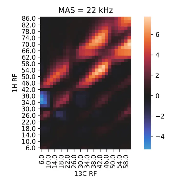 Heat map for $^{1}H$-$^{13}C$ Cross Polarization conditions.
What is Cross Polarization & why you want to do it?
Cross Polarization (CP) is a basic tool in solid state NMR first described by Hartmann & Hahn in 1962. In essence, we apply two simultaneous radiofrequency (RF) pulses to transfer magnetization from one nucleus to another. When the right frequencies (in the range of kiloHertz, kHz) are used, the respective nuclear resonances match and the transfer occurs under a so-called Hartmann-Hahn condition. One reason to do this is to boost the signal of an insensitive type of nucleus (e.g. $^{13}C$) by transferring the magnetization from a more polarizable one (e.g. $^{1}H$).
The 1-dimensional $^{1}H-^{13}C$ CP experiment is a common starting point for protein structure investigations with solid state NMR. It looks like this for a small model protein:
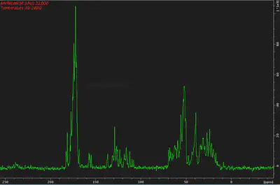
In this spectrum, we detect $^{13}C$ magnetization initially transferred from nearby $^{1}H$ via CP. The more efficient the CP step the stronger the signal, which for example enables shorter experiment times.
In the case here I wanted to maximize the backbone carbonyl signals, that’s the sharp peaks on the left side, around 175 ppm.
How do you do cross polarization?
In solid state NMR we usually rotate our sample very fast, at tens thousands of times per second (kHz again). This is called Magic Angle Spinning (MAS), and makes the Hartmann-Hahn conditions multiple and periodic, so there are several possible pairs of RF frequencies to choose from.
In practice you spin up you sample, set the RF values to a known CP condition and then,
because of experimental variability, you fine tune them. Topspin, the de facto only
program for acquisition of NMR experiments, has a routine called popt to fix one RF
and vary the other stepwise $n$ times over a given range. In the example, a 1D
spectrum is acquired at each $^{1}H$ RF:
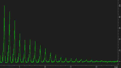
This example illustrates the periodicity of the CP conditions, with multiple local maxima.
Mapping the Hartmann-Hahn conditions
A one parameter optimization is often enough to get a good CP condition, but sometimes you need to be more exhaustive. You may not be sure which condition will be best, so you can do a 2-parameter optimization on both RF pulses.
This is handled by Topspin as a recursive popt over a new array of $m$ steps. The
implementation is a bit weird, so you end up with a 1D $m*n$ array of spectra indexed
by the experiment number for each $^{1}H$, $^{13}C$ RF pair. The best pair of
parameter values is recorded in the end according to the maximum integral or intensity
fo the signal.
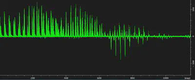
This representation of the data has two problems. First, the concatenated array does not display the second dimension intuitively. Secondly, the experiment number in the x axis does not give a quick idea of the respective RF values. The underlying structure of the data is totally obfuscated.
A heat map works best here
An obvious choice for representing an intensity that depends on two parameters is a heat
map. Python’s Seaborn has nice heat maps that work
seamlessly with Pandas, which can easily parse Topspin’s
popt results file (by default popt.protocol.999) to tabular format. The file contains the respective values of the RF pulses, and the maximum, minimum and integral of the signal in each experiment. The integral is our value of interest here.
import pandas as pd
import seaborn as sns

# Parse popt array data with pandas
popt = pd.read_csv(filepath_or_buffer="../data/expfolder/expno/popt.protocol.999",
                   skiprows=24,
                   skipinitialspace=True,
                   skipfooter=3,
                   sep="\s+",
                   engine="python",
                   index_col=0,
                   names=["1H RF",
                          "13C RF",
                          "max",
                          "min",
                          "integral"])

# Normalize integral values
popt["integral"] = popt["integral"]/popt["integral"].mean()
# Re-shape array for Seaborn
poptarray = popt.pivot(index="1H RF",
                       columns=["13C RF"],
                       values="integral")

# Plot with Seaborn
ax = sns.heatmap(poptarray,
                 cmap="icefire",
                 xticklabels=2,
                 yticklabels=2,
                 center=0)
ax.invert_yaxis()
ax.set_aspect(1)
ax.set_title("MAS = 22 kHz");
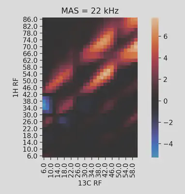
This approach gives a clear-cut representation of the Hartmann-Hahn condition landscape. One can immediately see the periodicity imposed by the MAS frequency in the distance between maxima (22 kHz in this example). The intensities of the different maxima can be readily compared. Moreover, the existence of different kinds of CP, one giving a positive signal and the other negative, becomes evident. In this case, this helped me find a CP condition (54 & 42 kHZ) which gave a very efficient transfer in a lower power range than I initially anticipated (~ 75 kHz for $^{1}H$).